In this article, I will show step by step how you can create and apply a data filter based on the font color of your data values. As an example, I am going to take a small set of hypothetical temperature data, then create and apply a data filter based on the font color of the data points then finally remove the filter. For the sake of this example, I am going to use blue font color to represent cold temperatures, green color to represent pleasant temperatures, and red to represent hot temperatures. Let’s get started first with creating and applying the filter.
Creating and applying a data filter based on font color in Google Sheets
Step 1: First visit Google Sheets and start a blank sheet. Step 2: Prepare two data columns by the names of “Days” and “Temperature” in columns D and E respectively, and fill in the data as shown in the reference figure. Step 3: Change the font colors of the different temperature values, as explained earlier.
Step 4: Once the data is ready, we are all set to create the filter. Select the range of data you want to apply the filter to. As per our example, this data is in column E. Step 5: Next, click on the “Data” menu and then on the “Create a filter” option.
Step 6: You will notice that a small upside-down triangle has appeared in the selected cell.
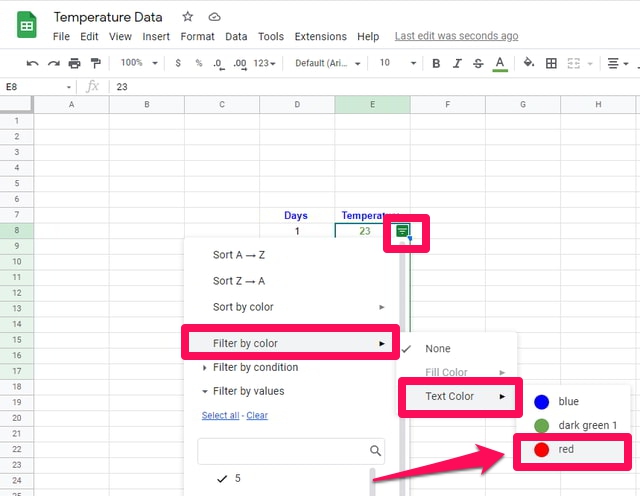
Step 7: Click on this triangle, a dropdown menu will appear giving you the different criteria you can use to sort or filter your data. Step 8: In the dropdown menu, point the cursor to the “Filter by color” option and then to the option “Text color”. Step 9: You will notice that Google Sheets have automatically detected the different font colors available in the selected data. Step 10: Click on the desired font color according to which, you want to sort your data. For this article, I am using the red color for sorting the sample data.
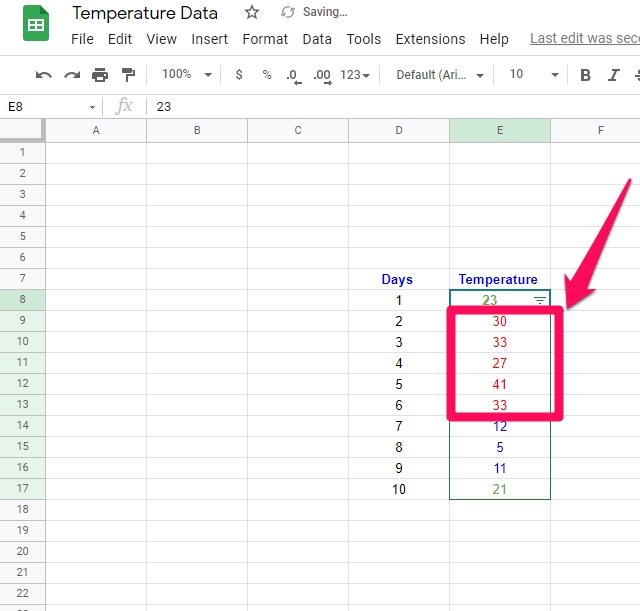
Step 11: After you have successfully applied the filter, you will notice that all the data points have been grouped that have the same color as chosen by you to filter the data. In my example, all data points having red color font are now grouped together.
Removing the created filter in Google Sheets
After you have created and applied a sorting filter to your data, a need for removing this filter might arise. Therefore, to do so, follow the following simple steps. Step 1: Click on the “Data” menu, a dropdown menu will appear. Step 2: In the dropdown menu, click on “Remove filter”.
Step 3: That’s it, you have successfully removed the earlier created filter, and you will notice that the inverted triangle is not there anymore.
Wrapping Up
In this article, I have shown step by step the process of creating a data filter based on the font color of the data, and then removing that filter in Google Sheets. A small set of hypothetical temperature data with different color fonts is used as an example. Use the same process to create a data filter based on the background color of the cells in Google Sheets, and share with us your experience in the comments section.